Photon Mapping: What It Is, How It Works & Why AI Matters

Realistic lighting is one of the most computationally demanding problems in computer graphics. Every convincing reflection and refraction requires approximating a recursive equation with no analytical solution. Among the early breakthroughs that made this practical, photon mapping introduced a structured way to handle complex light transport.

Modern rendering relies on GPU-accelerated path tracing and AI-driven lighting. Still, it remains grounded in the same physical framework defined decades ago.

In the following sections, photon mapping is examined within this computational context, its mathematical basis, its role in approximating the rendering equation, its relationship to path tracing, and its relevance in modern AI-driven architectural workflows.

What Is Photon Mapping?

Photon mapping is a two-pass global illumination algorithm developed by Henrik Wann Jensen to approximate the rendering equation in complex lighting scenarios. It was designed to simulate light transport effects that are difficult to capture efficiently with camera-based sampling alone, particularly caustics and indirect illumination.

In the first pass, discrete packets of light energy called photons are emitted from light sources and traced through the scene. Each surface interaction is stored in a spatial data structure, typically a KD-tree, forming the photon map.

In the second pass, rays are traced from the camera, and surface radiance is estimated by gathering nearby stored photons using density estimation. Instead of recalculating every light interaction at render time, the algorithm reuses previously recorded energy.

By tracing energy from the light source rather than relying solely on random camera sampling, photon mapping efficiently captures concentrated light effects.

For example, sunlight refracting through a glass façade can form sharp light patterns on a stone floor. The method trades additional memory and precomputation for improved stability in handling complex light interactions.

The Rendering Equation and the Cost of Light Simulation

All physically correct rendering techniques attempt to approximate the rendering equation, introduced by James Kajiya in 1986. This equation describes how light leaves a surface as a combination of emitted light and reflected incoming light integrated over a hemisphere.

Each term represents a physically meaningful quantity:

• Lₒ represents outgoing radiance toward the viewer

• Lₑ represents emitted radiance from the surface

• Lᵢ represents incoming radiance from other directions

• fᵣ represents the bidirectional reflectance distribution function that models material response

• ωᵢ · n represents the cosine term accounting for the angle between incoming light and the surface normal

The equation is recursive, meaning each incoming radiance term depends on other surfaces that follow the same rule. As a result, realistic rendering becomes a high-dimensional integration problem.

There is no closed-form analytical solution. Rendering engines approximate the equation using stochastic methods such as Monte Carlo sampling or density-based techniques such as photon gathering.

The computational cost rises quickly because:

• Every additional light bounce multiplies the number of possible light paths, especially in scenes with glossy or reflective materials.

• Transparent materials require accurate refraction simulation, which increases path complexity.

• Physically based rendering systems must respect energy conservation, requiring precise BRDF evaluation.

• Caustics represent rare but concentrated energy paths that are difficult to capture through random sampling alone.

As scene complexity increases, the number of potential light paths grows exponentially. Consequently, realistic lighting demands substantial computational resources.

Russian Roulette in Photon Tracing

During photon tracing, each surface interaction can produce reflected, transmitted, or absorbed energy. Naively spawning new photons for every possible event would cause exponential growth in photon count. After only a few bounces, the number of traced photons would become computationally infeasible.

To control this growth, Russian roulette is used as a probabilistic termination strategy. Instead of splitting photons into multiple branches, the algorithm randomly selects one outcome based on material reflectance and transmission probabilities. If the photon survives, its energy is appropriately scaled to maintain unbiased energy distribution in expectation.

This approach keeps the photon map populated with photons of comparable power and prevents excessive growth of deep multi-bounce paths. Although Russian roulette increases variance, it ensures convergence as the number of photons increases and keeps photon tracing computationally manageable.

What Gets Stored in the Photon Map?

Not every photon-surface interaction is stored. Photons are recorded only when they strike diffuse or non-specular surfaces. Storing photons on perfectly specular surfaces would provide no useful density information, since mirror and refraction events are better handled through deterministic ray tracing during the rendering pass.

For each stored photon, the photon map records:

• The surface position

• The incoming photon direction

• The photon power or flux contribution

  
  

A single photon may be stored multiple times along its path if it interacts with multiple diffuse surfaces. These stored interactions form the dataset used later for density-based radiance estimation.

This selective storage strategy ensures that the photon map represents meaningful diffuse energy distribution rather than deterministic specular reflections.

Biased vs Unbiased Estimators in Global Illumination

Photon mapping is considered a biased estimator because it approximates radiance using density estimation over a finite search radius. The result depends on photon count and gathering parameters.

Path tracing, by contrast, is an unbiased Monte Carlo estimator. As the number of samples approaches infinity, it converges to the true solution of the rendering equation in expectation. In practice, finite sample counts introduce variance, which appears as noise in the rendered image.

In practice:

• Biased methods often converge faster for rare light events but introduce approximation error due to density estimation.

• Unbiased methods converge to the correct solution in expectation as the number of samples increases, but finite sample counts introduce variance that appears as noise in the rendered image.

Variance reduction strategies such as importance sampling, stratified sampling, and multiple importance sampling are often applied to improve convergence efficiency.

Photon Mapping and Caustics Efficiency

Caustics are concentrated light patterns produced when light is reflected or refracted by specular materials. They often appear as bright, focused patches formed by glass, water, or polished surfaces.

Typical examples include:

• Sunlight refracting through pool water and forming dynamic patterns on the floor

• Glass façades projecting curved light bands into interior spaces

• Crystal luminaires producing sharp, concentrated highlights

These effects correspond to rare but visually dominant light paths. Because they represent statistically low-probability events, they are difficult to resolve efficiently with purely random sampling methods.

Photon mapping addresses this challenge by tracing energy directly from the light source and storing photon interactions during a pre-computation stage. During final shading, it performs localized radiance estimation by gathering nearby photons, allowing concentrated light patterns to be reconstructed more reliably.

This efficiency, however, introduces trade-offs:

• Increased memory consumption due to photon storage

• Parameter-dependent bias in density estimation

• Additional precomputation time before final rendering

• Potential smoothing artifacts if photon density is insufficient

Multiple Photon Maps: Global vs Caustic Maps

In practical implementations, photon mapping often uses multiple photon maps to separate different light transport components.

A global photon map stores photons that contribute to diffuse interreflection across the scene. A separate caustic photon map stores photons that have undergone specular interactions before reaching a diffuse surface. This separation improves efficiency because caustics require higher photon density to resolve sharp light concentrations.

Some extensions also introduce photon maps for participating media or volumetric scattering, enabling the simulation of subsurface scattering and light interaction within translucent materials.

By splitting photon storage into specialized maps, the rendering pass can estimate each light transport component more efficiently and with better control over quality.

When Should You Use Photon Mapping Today?

While path tracing dominates most modern production pipelines, photon mapping remains advantageous in scenes where light transport is governed by rare but high-energy interactions, particularly sharp caustics.

Because it traces energy from light sources first, it can more directly capture low-probability paths that are difficult to resolve efficiently through purely camera-driven sampling.

It is particularly effective when scenes include:

• Strong caustics from glass, water, or crystal materials

• Complex multi-bounce indirect illumination in enclosed architectural spaces

• Sharp specular-to-diffuse transitions where small subsets of paths carry significant energy

• Lighting configurations where path discovery is more challenging than noise reduction

In such cases, photon mapping can achieve stable caustic reconstruction with fewer camera samples compared to standard Monte Carlo path tracing. In offline workflows where additional memory usage and precomputation are acceptable, it may converge faster for caustic-heavy lighting setups.

However, for large-scale GPU-accelerated production rendering combined with denoising pipelines, path tracing often remains more scalable, easier to parallelize, and simpler to integrate into existing workflows.

In practice, photon mapping today is most relevant for specialized caustics problems, research applications, educational contexts, and hybrid rendering techniques rather than as a default solution for general-purpose architectural visualization.

Photon Mapping vs Modern Light Transport Techniques

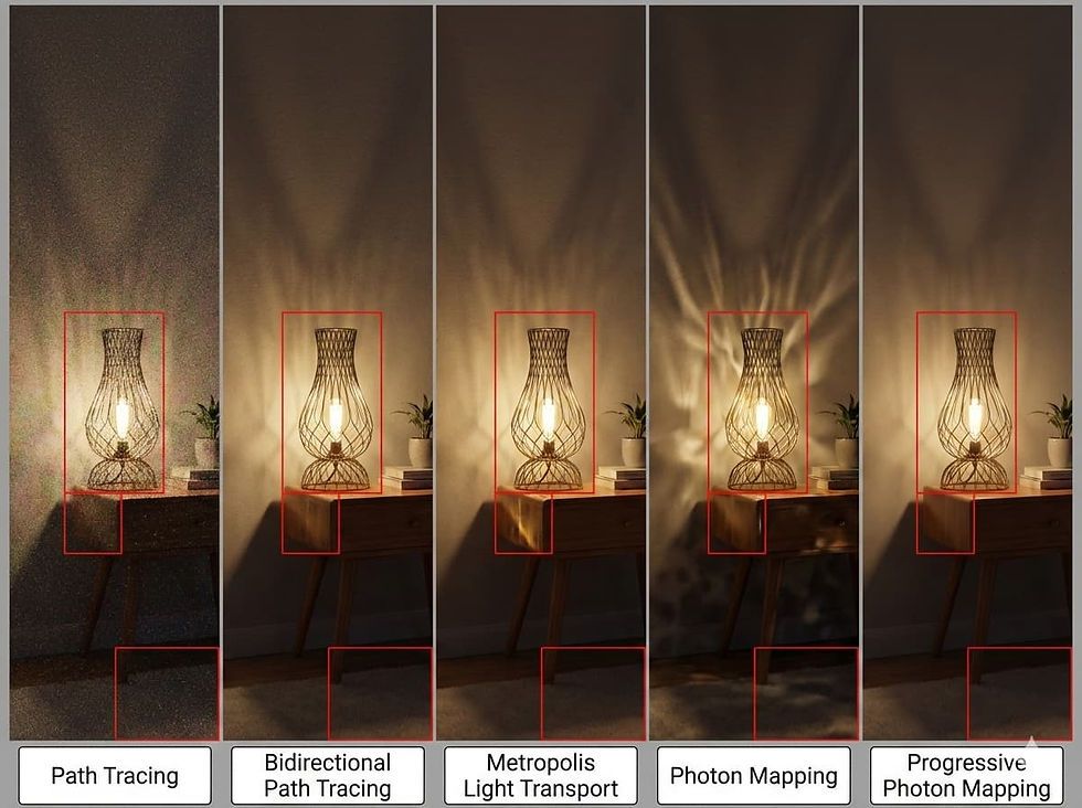
Path tracing remains dominant due to scalability and GPU acceleration. However, several advanced techniques improve convergence:

• Bidirectional path tracing constructs light transport paths from both the camera and the light sources, increasing the probability of capturing rare but high-energy interactions such as caustics.

• Metropolis light transport applies Markov chain sampling to explore important light paths more efficiently, concentrating computational effort on high-contribution regions of the solution space.

• Importance sampling biases sampling toward directions that contribute more energy, improving convergence speed and reducing variance in indirect lighting.

• Variance reduction techniques minimize noise while preserving physical accuracy, allowing faster convergence without increasing sample counts proportionally.

• Spectral rendering simulates light transport per wavelength rather than in simplified RGB space, enabling more physically accurate color interaction and dispersion effects.

Below is a simplified comparison:

Modern engines such as V-Ray, Arnold, and Blender Cycles primarily rely on GPU-accelerated path tracing combined with denoising.

A broader discussion of lighting principles and production workflows is explored in our guide to architectural rendering techniques and visualization pipelines.

Progressive Photon Mapping and Modern Variants

Standard photon mapping relies on a fixed photon count and a predefined gathering radius. This introduces bias that depends on density estimation parameters. To address these limitations, Progressive Photon Mapping (PPM) was developed as an iterative refinement approach.

Instead of computing a single photon map, PPM progressively emits additional photons over multiple passes. After each iteration, the photon gathering radius is reduced while the photon count increases. This gradual shrinkage improves consistency and reduces bias in radiance estimation.

As the number of iterations grows, the solution converges closer to the rendering equation while maintaining the stability benefits of photon density estimation. Unlike classic photon mapping, which may exhibit smoothing artifacts if under-sampled, PPM provides more predictable refinement behavior.

Modern variants also incorporate:

• Adaptive radius control for improved convergence

• GPU acceleration for photon tracing and storage

• Hybrid approaches combining photon mapping with path tracing

• Integration with bidirectional sampling strategies

Although path tracing dominates many production pipelines today, progressive photon techniques remain relevant in research environments and in scenes involving strong caustics or complex light transport.

Photon Mapping, PBR, and Energy Conservation

Physically based rendering is grounded in energy conservation, meaning surfaces cannot reflect more light than they receive. It relies on physically accurate BRDF models and microfacet theory to describe how materials respond to light at different angles.

Both photon mapping and path tracing operate within this same framework. Although they differ computationally, they approximate light transport while preserving realistic material behavior.

These techniques are not separate philosophies, but different implementations of the same physical laws. A deeper exploration of material realism and physically correct shading can be found in our overview of physically based rendering fundamentals.

Photon Mapping in the Era of AI Lighting Models

AI-driven lighting models change where computation happens. Instead of solving the rendering equation during every frame, neural networks learn statistical approximations of physically simulated light transport from datasets generated by path tracing and global illumination systems.

Rather than explicitly solving the rendering equation at runtime, modern AI systems transform lighting rendering into a learned inference problem based on physically simulated data.

For example, a network trained on thousands of glass-heavy interior scenes can reproduce convincing caustics and indirect illumination without explicitly tracing recursive light paths.

This shift significantly reduces runtime cost:

• No photon storage during image generation

• No extremely high Monte Carlo sample counts

• No recursive light transport evaluation at inference time

• Faster iteration during early architectural design

The result is not the abandonment of physics, but a redistribution of computational effort across the rendering pipeline.

ArchiVinci and Physics-Aware AI Lighting

AI lighting models often raise a critical question: "Are we replacing physics with approximation?"

In practice, platforms like ArchiVinci operate on a different computational layer while remaining grounded in physically based principles. Rather than solving the rendering equation during each iteration, ArchiVinci leverages neural models trained on physically accurate global illumination data.

Traditional render engines simulate full light transport at runtime. ArchiVinci shifts much of that computational load into pre-trained neural representations. The visual realism still originates from datasets generated through path tracing, global illumination techniques, and physically correct material models.

For early-stage architectural concept development, this enables rapid iteration on façade systems, glazing ratios, daylight penetration, interior materials, and lighting mood without waiting for high sample convergence.

ArchiVinci doesn't replace physics-based rendering. It enables faster iteration by leveraging models trained on physically simulated lighting data.

Why This Matters in Architectural Visualization?

In architectural workflows, rendering serves different purposes. Early-stage concept design prioritizes speed and iteration, while final marketing visuals demand higher physical accuracy.

AI lighting systems accelerate exploratory design by reducing computational friction. Physically based path tracing remains essential for validation-level realism and high-end production outputs.

The transition from photon mapping to AI-driven lighting doesn't signal the end of physics-based rendering. It reflects a shift in when and how computational effort is invested across the design pipeline.

Key Takeaways

• Realistic lighting is computationally expensive because it requires approximating a recursive light transport equation.

• Photon mapping solves this by tracing light from sources first, storing photon interactions, and reusing that information during rendering.

• It is especially strong at handling caustics and complex indirect lighting, where rare light paths are difficult to capture with pure random sampling.

• Photon mapping is a biased method, while path tracing is unbiased in expectation but often noisier at low sample counts.

• Progressive variants and multiple photon maps improve stability and convergence in challenging scenes.

• Today, path tracing dominates production pipelines, but photon mapping remains useful in caustic-heavy or specialized scenarios.

• AI lighting models shift computation from runtime to training time by learning patterns from physically simulated data.

• Platforms like ArchiVinci build on physically based principles while enabling faster iteration in architectural workflows.

• The shift from photon mapping to AI doesn't replace physics. It changes where and how computation happens.

Frequently Asked Questions

What is the difference between radiance and irradiance in photon mapping?

In photon mapping, radiance refers to light leaving a surface in a specific direction, while irradiance measures the total incoming light energy arriving at a surface from all directions. Photon density estimation often begins by approximating irradiance, which then contributes to the final radiance calculation.

Why are photons stored only on diffuse surfaces in photon mapping?

Photons are stored primarily on diffuse surfaces because density estimation requires a stable spatial distribution of light energy. Perfectly specular surfaces such as mirrors or ideal glass do not produce meaningful density patterns, so those interactions are handled through deterministic ray tracing instead.

What is a KD-tree?

A KD-tree is a spatial data structure used to organize points in multi-dimensional space for efficient nearest neighbor and range searches. In rendering, it is commonly used to quickly find nearby photons during photon mapping and global illumination calculations.

How does k-nearest neighbor search improve photon mapping accuracy?

Photon mapping often uses a k-nearest neighbor search to gather the closest photons around a shading point. This adaptive method adjusts the effective search radius based on photon density, improving stability and reducing estimation artifacts in global illumination.

Why is a KD-tree used for photon map storage?

A KD-tree enables efficient spatial indexing and fast nearest-neighbor queries. Since photon lookup performance directly affects rendering speed, KD-trees significantly improve the scalability of photon mapping in complex scenes.

What causes blurring artifacts in photon mapping renders?

Blurring artifacts occur when the photon gathering radius is too large or when photon density is insufficient. Because radiance is estimated using density over an area, sparse photon distributions can smooth out sharp lighting features such as fine caustics.

How does Russian roulette improve efficiency in photon tracing?

Russian roulette is a probabilistic termination strategy used during photon tracing to prevent exponential growth of light paths. By randomly terminating some photon paths and scaling the energy of surviving photons, the algorithm maintains energy conservation in expectation while keeping computation manageable.

Why is photon mapping considered a biased global illumination algorithm?

Photon mapping is classified as biased because it estimates radiance using density approximation over a finite radius. While this introduces systematic error, increasing photon count and refining the gathering radius allows the solution to approach the rendering equation over time.

How do diffusion models generate realistic lighting?

Diffusion models generate realistic lighting by learning patterns from physically based renders and progressively refining noise into images that match those learned light distributions, without explicitly solving the rendering equation.

Why are global and caustic photon maps separated in rendering engines?

Rendering engines often separate global and caustic photon maps because caustics require significantly higher photon density to resolve sharp light concentrations. This separation improves efficiency and provides better control over reconstruction quality.

How do AI lighting models differ from photon mapping?

AI lighting models do not trace and store photons during rendering. Instead, they learn statistical patterns of light transport from datasets generated by physically based renderers. Photon mapping explicitly simulates and records light interactions, while AI models approximate lighting outcomes through neural inference.

Do AI lighting systems solve the rendering equation?

No. AI lighting systems do not explicitly solve the rendering equation at inference time. They approximate the visual results of physically simulated light transport by learning from path-traced and global illumination training data.

Can AI-generated lighting reproduce caustics accurately?

AI models can generate visually convincing caustics if trained on similar lighting scenarios. However, unlike photon mapping or path tracing, they don't guarantee physically exact light transport or strict energy conservation.

When should AI lighting be preferred over photon mapping?

AI lighting is typically preferred during early-stage architectural design workflows where speed and rapid iteration are more important than strict physical validation. Photon mapping and path tracing remain better suited for physically accurate final production renders.

How does ArchiVinci maintain physically grounded lighting realism?

ArchiVinci uses neural models trained on physically accurate global illumination data. Although it doesn't simulate light transport at runtime, its outputs are informed by datasets generated through path tracing and physically based rendering systems.